Large datasets of fossil occurrences, often downloaded from online community-maintained databases (e.g. the Paleobiology Database), are a vital resource for understanding broad-scale evolutionary patterns, such as how biodiversity has changed through time and space. Such datasets, however, are often messy and must be ‘cleaned’ of inaccurate, incomplete, or duplicate data prior to analysis (see ‘ten rules’ Jones et al., 2025), as well as prepared and structured in a way that is suitable for the analysis being implemented.
Most palaeobiological analyses begin with routine but essential tasks, such as cleaning data, checking taxonomic names, binning occurrences in time or space, and reconstructing palaeogeographic distributions. The code to achieve such tasks is often rewritten from scratch for every project.
The palaeoverse R package aims to make such efforts more reusable, reproducible, and readable by:
replacing long, bespoke scripts with a few clear lines of code
using consistent function names, arguments, and outputs so that scripts are easy to follow and share
providing well-documented, tested, and peer-reviewed functions that are transparent and robust
2 Design
Three design choices shape how palaeoverse functions look and behave.
2.1 Built around occurrence data
Most functions in palaeoverse take an occurrence data.frame as input, so they directly fit the way many palaeobiologists already store their data.
NoteWhat is an occurrence dataset?
In an occurrence dataset, each row is a single record of something present at a particular place and time. That “something” is usually a taxon, but it does not have to be. For example, in palaeoverse’s in-built reefs dataset, each row is a fossil reef rather than a species.
Occurrence data typically include columns describing:
Identity, what the entity represents, such as taxonomy (e.g. accepted name, genus)
Age (e.g. maximum and minimum ages or named intervals)
Location (e.g. longitude and latitude)
Additional context (e.g. formation, collection, or reference)
It could look something a little like this:
occurrence_no
accepted_name
max_ma
min_ma
lng
lat
…
40163
Crocodylia
59.2
56
−74.68
39.97
…
40167
Gavialoidea
59.2
56
−74.68
39.97
…
40168
Gavialoidea
59.2
56
−74.68
39.97
…
…
…
…
…
…
…
…
2.2 Modular
Each function in palaeoverse does one job well. You can use one on its own, or chain several together into a full workflow:
# Load librarylibrary(palaeoverse)# Get example datadata(tetrapods)# Get time binsbins<-time_bins(interval ="Phanerozoic", rank ="stage")# Bin data temporallytetrapods|>bin_time(bins =bins, method ="mid")|># View first six rowshead()
Output
  occurrence_no collection_no                        identified_name
1        146665         12943     n. gen. Anconastes n. sp. vesperus
2        147090         13004                     Gorgonopsia indet.
3        147521         13043 n. gen. Procolophon n. sp. trigoniceps
4        147523         13044       n. gen. Ophiodeirus n. sp. casei
5        147563         13046         Broiliellus n. sp. arroyoensis
6        147564         13048              Broiliellus n. sp. olsoni
  identified_rank           accepted_name accepted_rank early_interval
1         species     Anconastes vesperus       species     Missourian
2        suborder             Gorgonopsia      suborder     Capitanian
3         species Procolophon trigoniceps       species         Induan
4         species       Araeoscelis casei       species     Artinskian
5         species Broiliellus arroyoensis       species      Kungurian
6         species      Broiliellus olsoni       species       Wolfcamp
  late_interval max_ma min_ma   phylum        class              order
1      Gzhelian 305.90  298.9 Chordata Osteichthyes      Temnospondyli
2          <NA> 265.10  259.9 Chordata Osteichthyes       Cotylosauria
3     Olenekian 252.17  247.2 Chordata     Reptilia NO_ORDER_SPECIFIED
4          <NA> 290.10  279.3 Chordata     Reptilia      Araeoscelidia
5          <NA> 279.30  272.3 Chordata Osteichthyes      Temnospondyli
6          <NA> 296.40  268.0 Chordata Osteichthyes      Temnospondyli
           family       genus abund_value  abund_unit        lng       lat
1    Trematopidae  Anconastes           2   specimens -106.34778  36.30444
2            <NA>        <NA>           1   specimens   22.00000 -32.36667
3 Procolophonidae Procolophon          10   specimens   26.50972 -32.10611
4   Araeoscelidae Araeoscelis           2 individuals  -98.93361  33.61167
5   Dissorophidae Broiliellus           6   specimens  -99.20000  33.80972
6   Dissorophidae Broiliellus           2   specimens  -98.14778  33.82639
                   collection_name cc     formation stratgroup member
1                  El Cobre Canyon US        Cutler       <NA>   <NA>
2            Hottentotsrivier Farm ZA Abrahamskraal   Beaufort   <NA>
3 Donnybrook (Queenstown District) ZA       Katberg   Beaufort   <NA>
4            Mouth of Godwin Creek US        Nocona    Wichita   <NA>
5               Broiliellus pocket US        Arroyo Clear Fork   <NA>
6                    Thaxton Ranch US          <NA>    Wichita   <NA>
                       zone   lithology1        environment
1                      <NA>    siltstone     dry floodplain
2 Tapinocephalus Assemblage    sandstone       "floodplain"
3                      <NA>     mudstone     fluvial indet.
4                      <NA> conglomerate terrestrial indet.
5                      <NA> not reported terrestrial indet.
6                      <NA> not reported terrestrial indet.
             pres_mode               taxon_environment        motility
1                 body brackish,freshwater,terrestrial actively mobile
2 body,mold/impression                     terrestrial actively mobile
3                 body                     terrestrial actively mobile
4                 body                     terrestrial actively mobile
5                 body brackish,freshwater,terrestrial actively mobile
6                 body brackish,freshwater,terrestrial actively mobile
       life_habit      diet id n_bins bin_assignment bin_midpoint
1 ground dwelling carnivore  1      2             39      301.300
2            <NA> carnivore  2      1             46      262.100
3            <NA>      <NA>  3      3             50      249.200
4            <NA>      <NA>  4      2             42      286.800
5 ground dwelling carnivore  5      2             43      278.225
6 ground dwelling carnivore  6      6             43      278.225
2.3 Flexible
Functions in palaeoverse are not tied to a single source such as the Paleobiology Database. Column names are arguments rather than fixed requirements. Therefore, data from any source can be used with ease providing you have the right data available.
# Load librarylibrary(palaeoverse)# Get example datadata(tetrapods)# Get unique speciestetrapods|>tax_unique(genus ="genus", family ="family", order ="order", class ="class", name ="accepted_name")|># View first six rowshead()
palaeoverse can be used for initial data exploration, as well as preparation for a wide range of downstream analyses, including diversity dynamics, macroevolution, macroecology and biogeography.
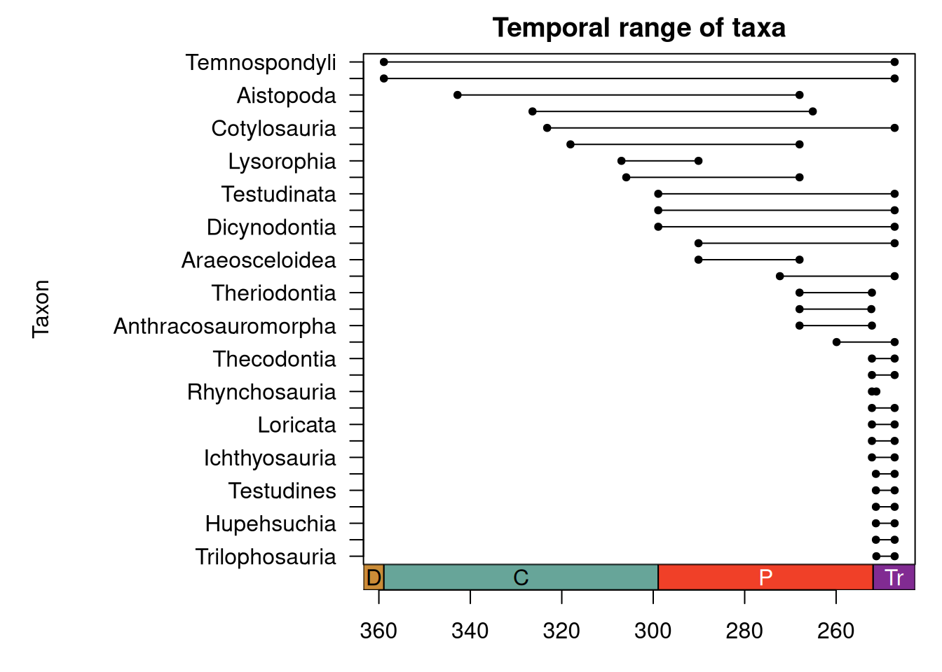
# Load librarylibrary(palaeoverse)# Get example datadata(tetrapods)# Estimate temporal range of taxatetrapods|># Drop NAssubset(!is.na(order))|># Plot temporal rangetax_range_time(name ="order", plot =TRUE)|># View first six rowshead()
Output
Temporal range of Carboniferous to Early Triassic tetrapods.
  r_number               name             formation   system         series
1        1   Tilkideligi Tepe                       Triassic Upper Triassic
2        2              Hydra Pantokrator Limestone Triassic Upper Triassic
3        3 Shiraho, W-Pacific                        Neogene       Holocene
4        4 Aksu-Terziler area                       Triassic Upper Triassic
5        5    Adnet, Salzburg                       Triassic Upper Triassic
6        6          Rotelwand                       Triassic Upper Triassic
        interval   biota_main       biota_sec      lng     lat country
1   lower Norian Calcisponges Stromatoporoids  30.3833 37.0333  Turkey
2  upper Carnian       Corals    Calcisponges  23.6333 37.3833  Greece
3         Recent       Corals           Algae 124.2500 24.3333 Pacific
4       Tuvalian Calcisponges Stromatoporoids  31.0333 37.8000  Turkey
5 upper Rhaetian       Corals    Calcisponges  13.1667 47.7000 Austria
6       Rhaetian       Corals    Calcisponges  13.1833 47.7000 Austria
                              authors
1                          Riedel, P.
2   Schafer, P., Senowbari-Daryan, B.
3 Kayanne, H., Suzuki, A. & Saito, H.
4                          Riedel, P.
5                         Schafer, P.
6                         Schafer, P.
                                                                                                                                                  title
1                                                 Riffbiotope im Karn und Nor (Obertrias) der Tethys: Entwicklung, Einschnitte und Diversitatsmuster. -
2                                                The Upper Triassic Pantokrator Limestone of Hydra (Greece): An example of a prograding reef complex. -
3                                                                      Diurnal changes in the partial pressure of carbon dioxide in coral reef water. -
4                                                 Riffbiotope im Karn und Nor (Obertrias) der Tethys: Entwicklung, Einschnitte und Diversitatsmuster. -
5  Fazielle Entwicklung und palokologische Zonierung zweier obertriadischer Riffstrukturen in den Nordlichen Kalkalpen (Oberrhat"-Riff-Kalke, Salzburg)
6 Fazielle Entwicklung und palokologische Zonierung zweier obertriadischer Riffstrukturen in den Nordlichen Kalkalpen (Oberrhat"-Riff-Kalke,  Salzburg)
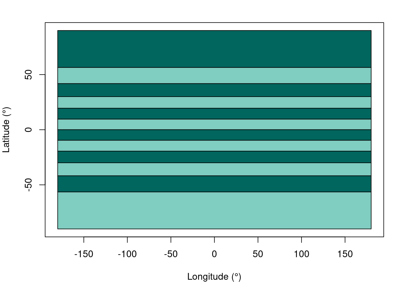
  year lat_bin  lat_max  lat_mid  lat_min
1 1990       3 41.81031 35.90516 30.00000
2 1982       3 41.81031 35.90516 30.00000
3 1995       4 30.00000 24.73561 19.47122
4 1990       3 41.81031 35.90516 30.00000
5 1979       2 56.44269 49.12650 41.81031
6 1979       2 56.44269 49.12650 41.81031
4 Reference guide
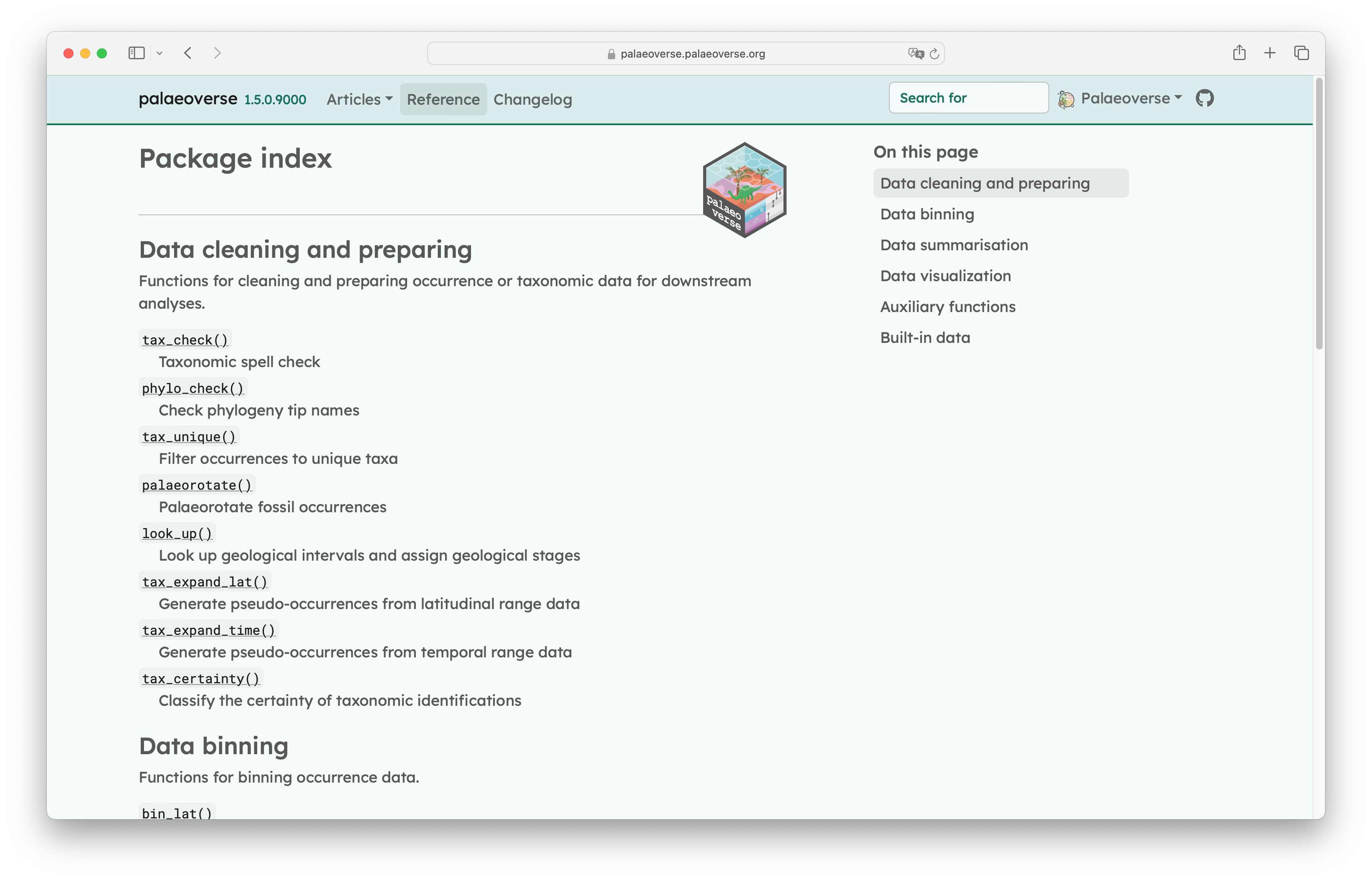
You can see all available functions and their documentation via the package’s dedicated website reference guide.
NoteWhere does palaeoverse fit?
Think of palaeoverse as the bridge between raw occurrence data and the analytical methods you want to apply, supporting the development of a full data prepration and exploration pipeline (see ‘ten rules’ Jones et al., 2025).
5 Getting help
Everyone gets stuck with using new tools from time-to-time, and knowing where to look for help is one of the most useful skills to develop. As with most R packages, palaeoverse has several layers of support, from built-in documentation to wider community support.
The palaeoverse website (https://palaeoverse.palaeoverse.org) hosts documentation for every function available, as well as vignettes (tutorials) demonstrating possible applications, and updates on new releases. It is a searchable resource and can be easier to navigate than the help pages in R.
If you are familiar with GitHub, you can search existing issues in the palaeoverserepository to see whether someone has previously encountered the issue you are facing and whether it has already been addressed. If you cannot find an answer, you are welcome to open an issue and include a minimal reproducible example (see guidance on writing one).
If you would like to request a new feature to be added to palaeoverse, or you think you have discovered a bug, you are invited to submit an issue on GitHub, following our contribution guide.
NoteJoin Zulip
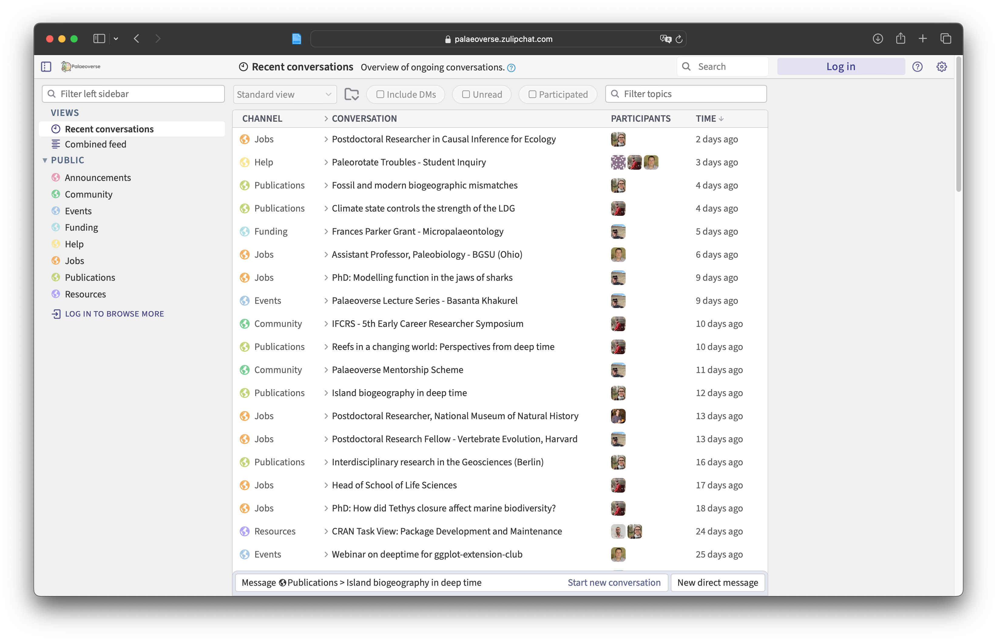
GitHub can be a daunting place if you have not used it before. You are welcome to join our Zulip and create a topic under “Help”.
You can joinpalaeoverse’s Zulip and ask for help if you are still stuck after reading the package documentation.
5.1 References
Jones, L. A., Dean, C. D., Allen, B. J., Drage, H. B., Flannery‐Sutherland, J. T., Gearty, W., Chiarenza, A. A., Dillon, E. M., Farina, B. M., & Godoy, P. L. (2025). Ten simple rules to follow when cleaning occurrence data in palaeobiology. Palaeontology, 68(5), e70028. DOI: 10.1111/pala.70028.