# Install palaeoverse
install.packages("palaeoverse")
# Load palaeoverse
library(palaeoverse)Tutorial 2: Tracking the diversity of early tetrapods
r
data
explore
prepare
How diverse were tetrapods in the Palaeozoic, and how was this diversity structured through time and across space?
Preamble
In this tutorial, you will use palaeoverse to explore the temporal and spatial diversity patterns of Palaeozoic tetrapods, using data from the Paleobiology Database (Uhen et al. 2026).
Along the way, you will meet many functions used in a typical palaeobiological workflow including exploring data, assigning a common time scale, binning occurrences, taxonomic wrangling, estimating palaeocoordinates, and summarising the results.
To help cement your knowledge, there are multiple exercises throughout this tutorial for you to work through.
NoteHow exercises work
- Questions: work out your answer in R first, then click the “Answers” box beneath the questions to check it.
-
Your turn: code chunks marked
___are incomplete. Replace each___before running them locally.
Introduction
The name Tetrapoda stems from the Ancient Greek words for ‘four’ and ‘feet’. It is a clade which originated when chordates first evolved limbs and developed the ability to walk, gradually transitioning from aquatic to terrestrial environments. All terrestrial four-limbed animals are members of this clade, including amphibians, reptiles, and mammals. This major evolutionary transition has received a lot of attention, in part because this clade represents our ancestors.
The fossil record of early tetrapods is considered relatively sparse, meaning that we do not have a clear picture of the timing and order of the acquisition of the different adaptations needed to thrive on land (e.g. Dunne et al. 2018). But just how sparse is the record, and what does it indicate about how diverse the earliest tetrapods were? Here, we will address the question “how did tetrapod diversity develop over the Palaeozoic?” by quantifying and comparing temporal and spatial diversity patterns.
Let’s start by installing and loading the palaeoverse R package:
The tetrapods dataset
In this tutorial, we will be using tetrapods for our analyses, an occurrence dataset of early tetrapods (n = 5270) drawn from the Paleobiology Database.
NoteBuilt-in datasets
Recall from the introduction that functions in palaeoverse are designed around the assumption that your data are stored in an occurrence data.frame, which is the expected input for almost all functions. The package includes two example occurrence datasets from different data sources: tetrapods and reefs.
Load the tetrapods dataset:
# Load built-in dataset
data(tetrapods)
Before conducting any analyses, it is always a good idea to explore your data first and understand what you are working with. Let’s take a look at the dataset:
# View dataset
View(tetrapods)
Note the structure of the dataset: each row contains a unique occurrence and each column contains a unique variable. Now we can get some more general information about what is contained in the dataset, such as the variable names and the types of data held for those variables:
# View column names
colnames(tetrapods)
Output
 [1] "occurrence_no"     "collection_no"     "identified_name"
 [4] "identified_rank"   "accepted_name"     "accepted_rank"
 [7] "early_interval"    "late_interval"     "max_ma"
[10] "min_ma"            "phylum"            "class"
[13] "order"             "family"            "genus"
[16] "abund_value"       "abund_unit"        "lng"
[19] "lat"               "collection_name"   "cc"
[22] "formation"         "stratgroup"        "member"
[25] "zone"              "lithology1"        "environment"
[28] "pres_mode"         "taxon_environment" "motility"
[31] "life_habit"        "diet"
# Inspect dataset structure
str(tetrapods)Output
'data.frame':   5270 obs. of  32 variables:
 $ occurrence_no    : num  146665 147090 147521 147523 147563 ...
 $ collection_no    : num  12943 13004 13043 13044 13046 ...
 $ identified_name  : chr  "n. gen. Anconastes n. sp. vesperus" "Gorgonopsia indet." "n. gen. Procolophon n. sp. trigoniceps" "n. gen. Ophiodeirus n. sp. casei" ...
 $ identified_rank  : chr  "species" "suborder" "species" "species" ...
 $ accepted_name    : chr  "Anconastes vesperus" "Gorgonopsia" "Procolophon trigoniceps" "Araeoscelis casei" ...
 $ accepted_rank    : chr  "species" "suborder" "species" "species" ...
 $ early_interval   : chr  "Missourian" "Capitanian" "Induan" "Artinskian" ...
 $ late_interval    : chr  "Gzhelian" NA "Olenekian" NA ...
 $ max_ma           : num  306 265 252 290 279 ...
 $ min_ma           : num  299 260 247 279 272 ...
 $ phylum           : chr  "Chordata" "Chordata" "Chordata" "Chordata" ...
 $ class            : chr  "Osteichthyes" "Osteichthyes" "Reptilia" "Reptilia" ...
 $ order            : chr  "Temnospondyli" "Cotylosauria" "NO_ORDER_SPECIFIED" "Araeoscelidia" ...
 $ family           : chr  "Trematopidae" NA "Procolophonidae" "Araeoscelidae" ...
 $ genus            : chr  "Anconastes" NA "Procolophon" "Araeoscelis" ...
 $ abund_value      : num  2 1 10 2 6 2 1 39 56 2 ...
 $ abund_unit       : chr  "specimens" "specimens" "specimens" "individuals" ...
 $ lng              : num  -106.3 22 26.5 -98.9 -99.2 ...
 $ lat              : num  36.3 -32.4 -32.1 33.6 33.8 ...
 $ collection_name  : chr  "El Cobre Canyon" "Hottentotsrivier Farm" "Donnybrook (Queenstown District)" "Mouth of Godwin Creek" ...
 $ cc               : chr  "US" "ZA" "ZA" "US" ...
 $ formation        : chr  "Cutler" "Abrahamskraal" "Katberg" "Nocona" ...
 $ stratgroup       : chr  NA "Beaufort" "Beaufort" "Wichita" ...
 $ member           : chr  NA NA NA NA ...
 $ zone             : chr  NA "Tapinocephalus Assemblage" NA NA ...
 $ lithology1       : chr  "siltstone" "sandstone" "mudstone" "conglomerate" ...
 $ environment      : chr  "dry floodplain" "\"floodplain\"" "fluvial indet." "terrestrial indet." ...
 $ pres_mode        : chr  "body" "body,mold/impression" "body" "body" ...
 $ taxon_environment: chr  "brackish,freshwater,terrestrial" "terrestrial" "terrestrial" "terrestrial" ...
 $ motility         : chr  "actively mobile" "actively mobile" "actively mobile" "actively mobile" ...
 $ life_habit       : chr  "ground dwelling" NA NA NA ...
 $ diet             : chr  "carnivore" "carnivore" NA NA ...
Details on the dataset (e.g. source) are also available via the usual documentation call:
# Get dataset documentation
help(tetrapods)
Let’s now generate some simple summary statistics, to help us understand the scope and scale of the dataset.
CautionExercise 1: Get to know
tetrapods
- How many occurrences (observations/rows) are there?
- How old is the oldest tetrapod occurrence?
- How young is the youngest occurrence in the dataset?
- Are any of the occurrences missing coordinates?
TipExercise 1: Answers
-
nrow(tetrapods): 5270 -
max(tetrapods$max_ma): 358.9 -
min(tetrapods$min_ma): 247.2 -
sum(is.na(tetrapods$lat)): 0
Time binning
In order to investigate diversity through time, we want to allocate each of our occurrences to a single time bin. First, we will generate stage-level bins spanning the Carboniferous and Permian, using palaeoverse::time_bins().
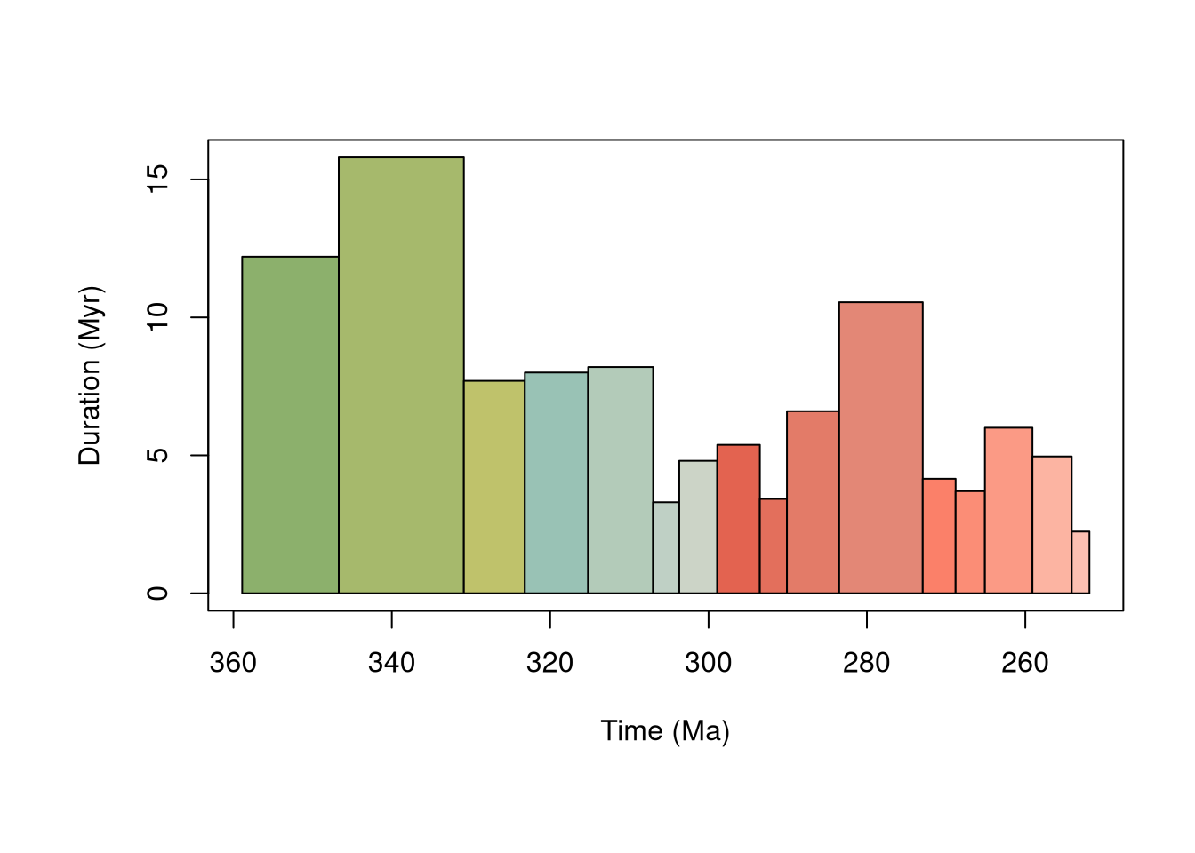
The function gives us the option to generate a plot of our time bins – here we can see some variation in the duration of our different stages, with particularly long stages in the Early Carboniferous and shorter ones across the Carboniferous–Permian boundary. This is a form of structure inherent to our dataset, and something we should bear in mind for our downstream analyses.
We can also take a look at the structure of the outputted table which describes the time bins.
# View first few rows
head(bins)
Output
  bin interval_name  rank max_ma mid_ma min_ma duration_myr abbr  colour  font
1   1   Tournaisian stage  358.9 352.80  346.7         12.2    T #8CB06C black
2   2        Visean stage  346.7 338.80  330.9         15.8    V #A6B96C black
3   3  Serpukhovian stage  330.9 327.05  323.2          7.7   Se #BFC26B black
4   4    Bashkirian stage  323.2 319.20  315.2          8.0    B #99C2B5 black
5   5     Moscovian stage  315.2 311.10  307.0          8.2    M #B3CBB9 black
6   6    Kasimovian stage  307.0 305.35  303.7          3.3   Ka #BFD0C5 black
In the Paleobiology Database, occurrences are allocated to named temporal intervals, with the numeric dates filled in using the Database’s internal timescale. We are going to generate numeric ages for these named intervals using palaeoverse::look_up(), to check whether these are up-to-date.
Output
  interval_max_ma interval_mid_ma interval_min_ma
1         307.000         302.950          298.90
2         265.100         262.100          259.10
3         251.902         249.551          247.20
4         290.100         286.800          283.50
5         283.500         278.225          272.95
6         293.520         281.160          268.80
CautionExercise 2: Check for updated ages
- How many different interval names are there in
tetrapods?
# Your turn: work out which columns contain the interval names
length(unique(c(tetrapods$___, tetrapods$___)))- How many interval names could not be matched using
look_up()? - What proportion of occurrences could a match not be found for?
# Your turn: which column can tell us this information?
(sum(is.na(___$___)) / nrow(___))
TipExercise 2: Answers
-
length(unique(c(tetrapods$early_interval, tetrapods$late_interval))): 74 - The warning message tells us that three interval names could not be matched: “Early Triassic, Late Pennsylvanian, Vokhmian”.
-
(sum(is.na(tetrapods$interval_max_ma)) / nrow(tetrapods)): 0.0301708
Now that we have an understanding of the amount of uncertainty surrounding the age of some of our occurrences, let’s tidy it up by filling in the ages of intervals not included in the look_up() table with those that they were allocated by the Paleobiology Database:
# Make sure that any values which could not be matched contain their original
# values
tetrapods$interval_max_ma <- ifelse(is.na(tetrapods$interval_max_ma),
                                    tetrapods$max_ma,
                                    tetrapods$interval_max_ma)
tetrapods$interval_min_ma <- ifelse(is.na(tetrapods$interval_min_ma),
                                    tetrapods$min_ma,
                                    tetrapods$interval_min_ma)
tetrapods$interval_mid_ma <- (tetrapods$min_ma + tetrapods$max_ma) / 2

# Check that there are no remaining NA values
sum(is.na(tetrapods$interval_max_ma))
Output
[1] 0Now we are ready to allocate our occurrences to our time bins. We will do this using the palaeoverse::bin_time() function. Here, for simplicity, we will use the “mid” method, which places each occurrence into the time bin corresponding to the midpoint between its maximum and minimum age.
However, first we need to rename our columns so we don’t accidentally use the old ages:
# Rename columns so that new intervals are used for binning
colnames(tetrapods)[which(colnames(tetrapods) == "max_ma")] <- "old_max_ma"
colnames(tetrapods)[which(colnames(tetrapods) == "min_ma")] <- "old_min_ma"
colnames(tetrapods)[which(colnames(tetrapods) == "interval_max_ma")] <-
  "max_ma"
colnames(tetrapods)[which(colnames(tetrapods) == "interval_min_ma")] <-
  "min_ma"
And then we can bin our data:
# Generate time bins
mid_tetrapods <- bin_time(occdf = tetrapods,
                          bins = bins,
                          method = "mid")
It seems we have hit an error!
CautionExercise 3: Spot the problem
Why are we getting an error when we try to bin our occurrences?
TipExercise 3: Answer
If we remember back to our initial exploration of the data, the youngest occurrences in the dataset are Early Triassic in age. This sits outside of the Carboniferous–Permian interval across which we have generated our time bins. The function is giving us an error because these Early Triassic occurrences are too young to be placed into any of the provided time bins.
We will remove these problematic occurrences and try again:
This time we have received a warning, but no error. Let’s take a look at the new columns added to the dataset:
Output
  id n_bins bin_assignment bin_midpoint
1  1      2              7      301.300
2  2      1             14      262.100
4  3      1             10      286.800
5  4      1             11      278.225
6  5      4             11      278.225
7  6      2              8      296.210
The second of these new columns is n_bins, which tells us how many stages are spanned by our occurrences. We can summarise this information to explore how bin_time has processed our data:
# Make a table of potential number of bins
table(mid_tetrapods$n_bins)
Output
   1    2    3    4    5    6    7    8
2401 530 177 216 12 21 5 16 Output
          1           2           3           4           5           6
0.710775607 0.156897573 0.052397869 0.063943162 0.003552398 0.006216696
          7           8
0.001480166 0.004736530
We can see that around 70% of the occurrences can be allocated to a single stage, whereas the remaining 30% span between 2 and 8 geological stages. For this 30%, the method that we choose to bin the data becomes very important, as it determines which of these stages the occurrence will be placed within.
Spatial binning
Remember at the start of the exercise, we saw that every occurrence has a latitude and longitude. However, this corresponds to the modern-day coordinates of the locality in which they were found. If we want to understand spatial patterns in deep time, we need to infer the palaeo-coordinates at which the fossils were deposited.
We can use palaeoverse::palaeorotate() to use a Global Plate Model (GPM) to infer how rocks on the Earth’s surface have shifted over time due to continental drift. You can find more information about how this works using help(palaeorotate). It’s worth noting that different GPMs will produce different results (Buffan et al. 2023), but for now we will go ahead with using the PALEOMAP GPM (Scotese & Wright 2018):
# Palaeorotate occurrences
mid_tetrapods <- palaeorotate(occdf = mid_tetrapods, age = "bin_midpoint",
                              method = "point", model = "PALEOMAP")
Let’s now take a look at our new columns containing the palaeocoordinates.
Output
     p_lng    p_lat
1 -39.1618   2.9214
2 -33.9023 -59.1946
4 -30.1811  -0.9483
5 -28.4255   2.7177
6 -27.6584   2.2973
7 -16.1476 -5.0776Output
[1] 0We can now generate our spatial bins and place our occurrences into them based on their palaeo-coordinates. Here we will generate and bin into equal-area hexagonal grid cells (based on Uber’s H3 system):
# Generate hex cells with a centroid spacing of ~100 km, and bin occurrences
mid_tetrapods <- bin_space(occdf = mid_tetrapods,
                           lng = "p_lng",
                           lat = "p_lat",
                           spacing = 100)
# Show the first 6 rows of the new columns added using `bin_space()`.
head(mid_tetrapods[, c("cell_ID", "cell_centroid_lng", "cell_centroid_lat")])
Output
          cell_ID cell_centroid_lng cell_centroid_lat
1 8380d4fffffffff         -38.83199          3.041113
2 83dd68fffffffff         -34.66666        -59.098482
4 837d4bfffffffff         -29.87896         -1.198269
5 837c45fffffffff         -28.90252          2.777952
6 837c44fffffffff         -27.94209          2.183584
7 837d85fffffffff         -16.18503         -5.090402
We can see that each occurrence has been placed into a grid cell, described using a unique ID, and with the centroid of the cell also provided.
Taxonomic wrangling
Fossil occurrence data are often messy, and the taxonomic information attached to them is no exception. Inspecting and cleaning these data is a fundamental step in ensuring that counts of unique taxa through time are accurate. For example, without it, the same species can be counted multiple times due to slight spelling differences. The palaeoverse::tax_check() function helps you find such issues by flagging similar chracter strings, which may potentially be spelling variants (or typos) of the same taxon. Variants are provided within alphabetical groups by default, or within higher taxonomic groups if these are provided:
# Check taxon names alphabetically
tax_check(taxdf = tetrapods, name = "genus", dis = 0.05)
Output
$synonyms
  group     greater     lesser count_greater count_lesser
1     D Dvinosaurus Dinosaurus            23            2
2     V   Varanopus   Varanops             5            3

$non_letter_name
NULL

$non_letter_group
NULL
In our tax_check() output, two pairs of genus names are flagged: Dvinosaurus/Dinosaurus and Varanopus/Varanops. Without any prior knowledge, it would be easy to assume that each pair is a spelling variant of the same name. However, on closer inspection, we can see that these are distinct genera belonging to different families:
Output
           genus          family
37   Dvinosaurus   Dvinosauridae
290     Varanops     Varanopidae
3940  Dinosaurus Phthinosuchidae
4704   Varanopus   Captorhinidae
If we inspect tetrapods again, this time grouping by family, no names are flagged, so we’re good to move on:
# Check taxon names by group
tax_check(taxdf = tetrapods, name = "genus", group = "family", dis = 0.05)
Output
$synonyms
NULL

$non_letter_name
NULL

$non_letter_group
[1] "NO_FAMILY_SPECIFIED"
Now that we know our taxonomic names are clean, we can start thinking about how to identify and count unique taxa. In many cases, palaeobiologists count unique taxa by retaining only unique occurrences identified to a given taxonomic resolution (e.g. genera or species); however, this can result in some useful information being discarded. The palaeoverse::tax_unique() function retains occurrences identified to a coarser taxonomic resolution which are not already represented within the dataset. Take, for example, the following occurrences:
- Albertosaurus sarcophagus
- Ankylosaurus sp.
- Ceratopsidae indet.
- Ornithominus sp.
- Tyrannosaurus rex
A filter for species-level identifications would reduce the species richness to just two (A. sarcophagus and T. rex). However, none of these clades are nested within one another, so each of the indeterminately identified occurrences represents at least one species not already represented in the dataset. tax_unique() is designed to deal with such taxonomic data and would retain all five ‘species’ in this example. For further details see help(tax_unique).
This function can be especially helpful when we want to quantify alpha (local) diversity. Let’s use this function to investigate the number of unique genera in our dataset.
# Filter occurrences to unique genera
tet_genera <- tax_unique(occdf = mid_tetrapods,
                         genus = "genus", family = "family",
                         order = "order", class = "class",
                         resolution = "genus")
# Get a preview of the output table
head(tet_genera)
Output
         class         order            family            genus
1 Osteichthyes  Dicynodontia              <NA>         Abajudon
2 Osteichthyes  Cotylosauria Charassognathidae        Abdalodon
3     Reptilia          <NA>  Nyctiphruretidae      Abyssomedon
4 Osteichthyes Temnospondyli      Zatracheidae Acanthostomatops
5 Osteichthyes Temnospondyli      Trematopidae         Acheloma
6 Osteichthyes          <NA>   Acherontiscidae    Acherontiscus
           unique_name
1         Abajudon sp.
2        Abdalodon sp.
3      Abyssomedon sp.
4 Acanthostomatops sp.
5         Acheloma sp.
6    Acherontiscus sp.
CautionExercise 4: Save our cryptic diversity
How many occurrences are retained in the dataset by tax_unique(), which would otherwise have been discarded?
# Your turn: calculate the number of unique genera in tax_unique output
length(unique(tet_genera$___))

# Now for the original dataset for comparison: what must not be counted?
length(unique(___.omit(mid_tetrapods$___)))
TipExercise 4: Answer
length(unique(tet_genera$unique_name)): 719
For the original dataset, we need to remember not to count values (i.e. genus names) that are NA.
length(unique(na.omit(mid_tetrapods$genus))): 716
This shows us that there are three additional unique genera retained when we use tax_unique.
We can see the additional occurrences retained at the end of our output table.
Output
           class        order           family genus             unique_name
717 Osteichthyes         <NA>  Acanthostegidae  <NA>  Acanthostegidae indet.
718 Osteichthyes Dicynodontia   Dicynodontidae  <NA>   Dicynodontidae indet.
719 Osteichthyes Dicynodontia Endothiodontidae  <NA> Endothiodontidae indet.
Now that we’ve seen what this function can do, let’s apply it in a way that lets us check for unique genera in each collection (= locality) using palaeoverse::group_apply():
# Find unique genera (with tax_unique) in each collection (using group_apply)
coll_genera <- group_apply(occdf = mid_tetrapods,
                           group = c("collection_no"),
                           fun = tax_unique,
                           genus = "genus",
                           family = "family",
                           order = "order",
                           class = "class",
                           resolution = "genus")

# See structure of the new dataframe
head(coll_genera)
Output
         class         order           family      genus         unique_name
1 Osteichthyes          <NA>             <NA>       <NA> Osteichthyes indet.
2 Osteichthyes Temnospondyli    Dissorophidae   Parioxys        Parioxys sp.
3 Osteichthyes  Cotylosauria             <NA>   Archeria        Archeria sp.
4     Reptilia          <NA>     Bolosauridae Bolosaurus      Bolosaurus sp.
5 Osteichthyes  Cotylosauria      Diadectidae  Diadectes       Diadectes sp.
6 Osteichthyes  Cotylosauria Sphenacodontidae Dimetrodon      Dimetrodon sp.
  collection_no
1         11149
2         11152
3         11165
4         11165
5         11165
6         11165
In addition to the columns we had before, we have now gained a collection_no column. We are now able to count the unique number of genera per collection.
# Calculate the number of unique genera per collection
coll_taxa <- group_apply(coll_genera, group = "collection_no", fun = nrow)

# Rename column names:
colnames(coll_taxa) <- c("n_taxa", "collection_no")

# Take a quick look at the new dataframe
head(coll_taxa)
Output
  n_taxa collection_no
1      1        104796
2      1        106270
3      3        106558
4      8        108766
5      3        109702
6      1         11149
In order to plot alpha diversity through time, we will also need to add interval age data to this table.
# Subset to collections and their ages in millions of years:
coll_info <- mid_tetrapods[, c("collection_no", "max_ma", "interval_mid_ma",
                               "min_ma")]

# Remove duplicated collections based on the collection number (column 1)
coll_info <- coll_info[!duplicated(coll_info[1]),]

# Combine this dataframe with the dataframe from above
alpha_data <- merge(coll_info, coll_taxa, by = "collection_no")

# Take a look:
head(alpha_data)
Output
  collection_no max_ma interval_mid_ma min_ma n_taxa
1         11149 290.10          284.70 283.50      1
2         11152 293.52          283.90 272.95      1
3         11165 298.90          294.50 290.10      9
4         11323 303.70          301.15 293.52      1
5         12943 307.00          302.40 298.90      1
6         12976 283.50          275.80 272.95      7
Great! Now we can plot our alpha diversity through time. Let’s start with a simple scatterplot:
# Make a plot for alpha diversity in the Carboniferous and Permian
plot(alpha_data$interval_mid_ma, alpha_data$n_taxa, # add the points
     xlim = rev(range(alpha_data$interval_mid_ma,
                      na.rm = TRUE)), # reverse the x-axis
     xlab="Time (Ma)", ylab="No. taxa", # axes labels
     pch = 19, col = "#0e826f") # point style and colour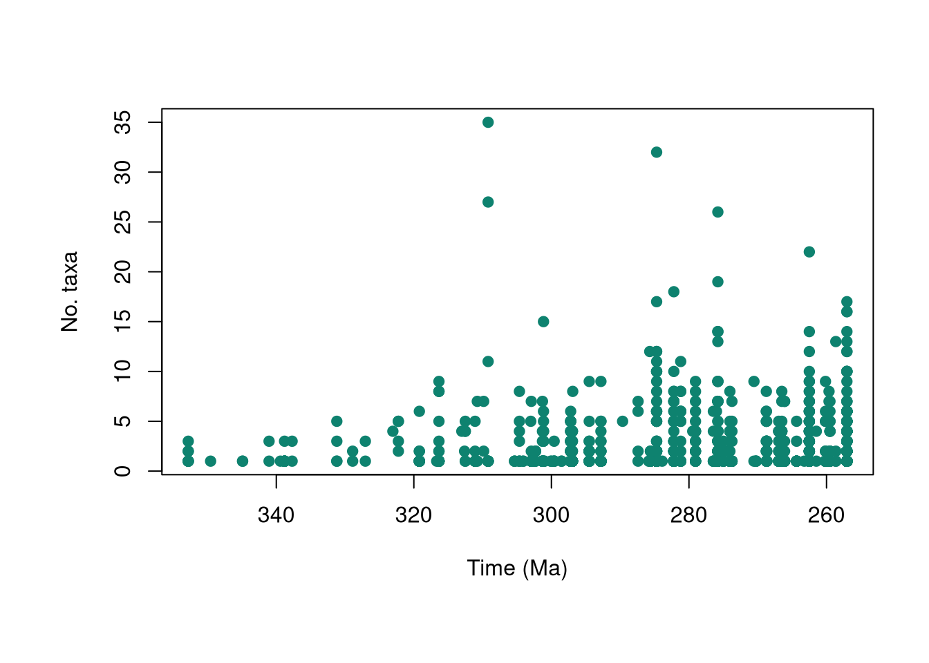
It’s a good start, but we would like to know which data points belong in which stages. We can use palaeoverse::axis_geo() to add a geological timescale to our plot.
# Set margins
par(mar = c(7.1, 4.1, 4.1, 2.1)) # expand at bottom if adding more intervals
# Make the final alpha diversity plot
plot(alpha_data$interval_mid_ma, alpha_data$n_taxa, # add the points
     axes = FALSE,
     xlim = rev(range(alpha_data$interval_mid_ma,
                      na.rm = TRUE)), # reverse the x-axis
     xlab = " ", ylab = "No. taxa", # axes labels
     pch = 19, col = "#0e826f") # point style and colour
box()
axis(2) # add a normal axis to the left side
axis_geo(side = 1, intervals = list("epochs", "periods"),
         title = "Time (Ma)")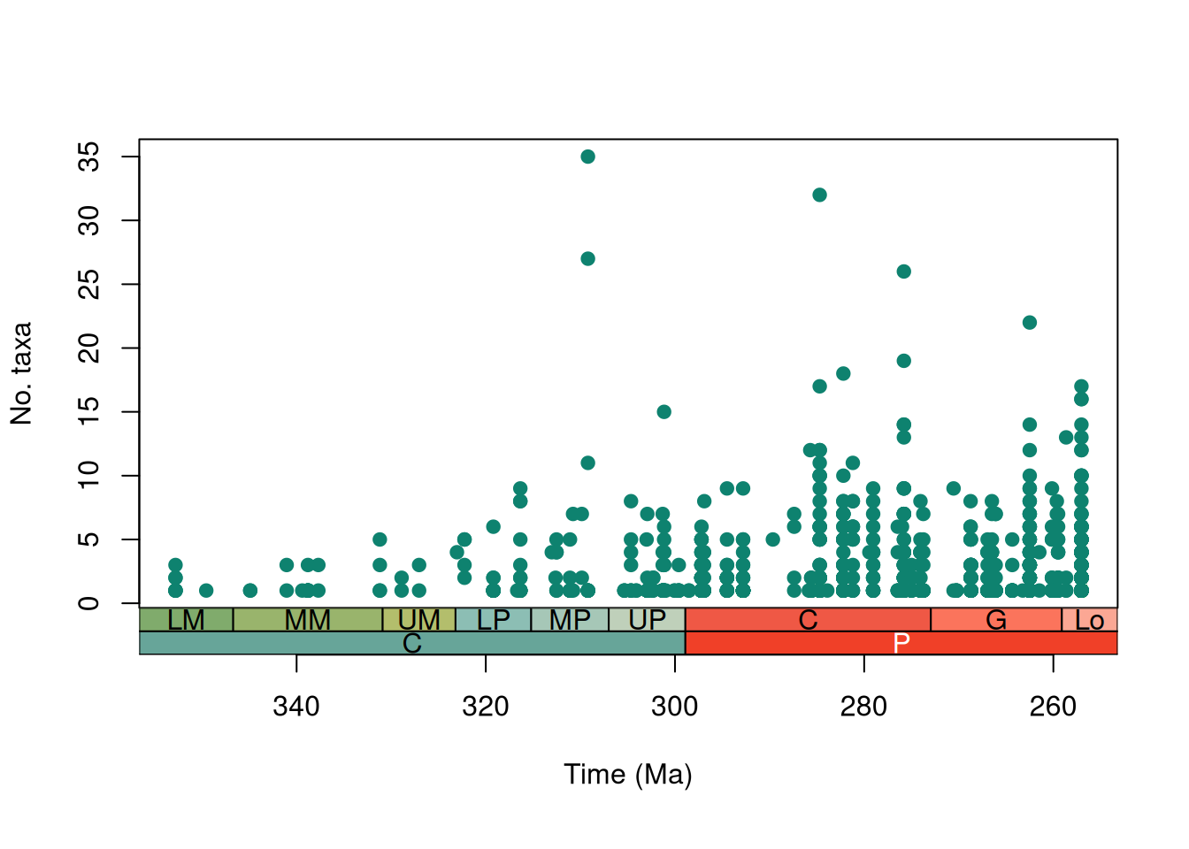
We can now see an overall increasing trend in maximum tetrapod alpha diversity over the Carboniferous and Permian, with a few extra-diverse outliers.
CautionExercise 5: Interrogating alpha diversity
What steps could we take to investigate this trend in alpha diversity further?
TipExercise 5: Answer
There are many things we could try, but here are some suggestions:
- Fit a trend line, to see whether the average alpha richness really increased
- Identify the overly-diverse (outlier) collections and look into why they were so diverse, do they represent Lagerstätten?
- Look into the relationship between stage duration and alpha diversity
- Explore the effect of the lower bound on this distribution - every locality contains at least one tetrapod, what impact does this have on the averages we might want to calculate?
Quantifying spatial patterns
Another factor that we can examine is how the range size of taxa changed across the Carboniferous-Permian boundary. We can examine this spatial distribution through time using the palaeoverse::tax_range_space() function, which provides several different methods for estimating the distribution of taxonomic occurrences. For now we’ll use the method con which calculates the geographic range of taxa using a convex hull, but the rest of the methods are described in detail in the function documentation which can be accessed via help(tax_range_space).
We can use this in combination with group_apply to calculate the convex hull size for each genus in each time interval:
# First, remove any occurrences without a genus
space_tetrapods <- subset(mid_tetrapods, !is.na(genus))
# Find temporal range of all genera
space_tetrapods <- group_apply(occdf = space_tetrapods,
                               group = c("bin_midpoint"),
                               fun = tax_range_space,
                               name = "genus",
                               lng = "p_lng",
                               lat = "p_lat",
                               method = "con")
# Have a look at the dataset
head(space_tetrapods)
Output
             taxon taxon_id      area bin_midpoint
1        Abdalodon        1      0.00       256.62
2        Acrodenta        2      0.00       256.62
3      Adelosaurus        3      0.00       256.62
4    Aelurognathus        4 292403.96       256.62
5     Aelurosaurus        5  11864.55       256.62
6 Aenigmastropheus        6      0.00       256.62
As you can see, the combination of group_apply and tax_range_space produces a dataset with the area of geographic range for each taxon in kilometers squared for each time interval.
CautionExercise 6: Area Zero
What does it mean for a convex hull to have an area of 0?
TipExercise 6: Answer
A value of 0 means the convex hull has no volume, because it consists of a single point - i.e. there is only a single occurrence of that genus in that time bin.
From this information we can now plot how the average range size of tetrapods changed throughout the Carboniferous and Permian:
# Find the average geographic range size for each time interval
space_tetrapods_mean <- group_apply(space_tetrapods, "bin_midpoint",
                                    function(df) mean(df$area))
colnames(space_tetrapods_mean) <- c("mean_area", "bin_midpoint")
# Create a plot of average range size through time
plot(space_tetrapods_mean$bin_midpoint,
     space_tetrapods_mean$mean_area,
     axes = FALSE,
     # reverse the x-axis
     xlim = rev(range(as.numeric(space_tetrapods_mean$bin_midpoint),
                      na.rm = TRUE)),
     # axes labels
     xlab = " ",
     ylab = expression("Average range size of tetrapod genera (km"^2*")"),
     pch = 19, col = "#0e826f") # point style and colour
box()
axis(2) # add a normal axis to the left side
axis_geo(side = 1, intervals = list("epochs", "periods"))
title(xlab = "Time (Ma)", line = 4)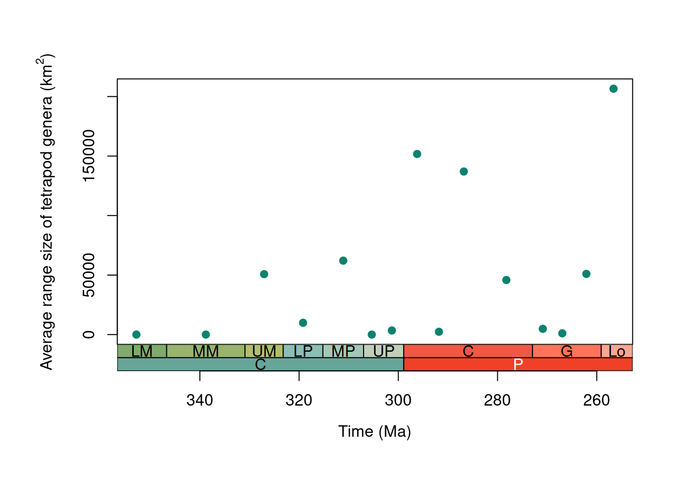
From this plot it seems like the average geographic range size of tetrapods increased during the Permian. However, we first need to be sure we’re not picking up on another pattern. Remember how we calculated the number of unique geographic cells in each time interval earlier? This provides a measure of the spatial spread of the fossil record. It might be that we’re not picking up on an increased range size, but just a larger geographic spread of fossil bearing rocks within the Permian. To see if this is the case, we can run a simple correlation test between the average geographic range size of tetrapods and the number of unique grid cells in each time interval:
# Calculate the number of unique cells in each time bin
unique_cells <- unique(mid_tetrapods[, c("bin_midpoint", "cell_ID")])
spat.cov <- group_apply(unique_cells, group = "bin_midpoint", fun = nrow)
# Run a correlation test between mean range size and the spatial spread of
# cells through time
cor.test(log10(space_tetrapods_mean$mean_area), log10(spat.cov$nrow),
         method = "spearman")
Output
    Spearman's rank correlation rho

data:  log10(space_tetrapods_mean$mean_area) and log10(spat.cov$nrow)
S = 189.34, p-value = 0.007191
alternative hypothesis: true rho is not equal to 0
sample estimates:
      rho
0.6618858
The high rho value and a p-value less than our cut off for significance (0.05) indicate a strong and statistically significant correlation between average geographic range size and the spatial spread of data. Seems like this work is far from over…
…but we’ll leave the rest to you!
Wrap-up
Hopefully this tutorial has shown you some of the potential uses of palaeoverse functions and helped provide a workflow for your own analyses.
In this tutorial, you have:
- explored an occurrence dataset and run functions across groups with
group_apply() - linked interval names to a common time scale with
look_up() - binned occurrences by time with
time_bins()andbin_time() - estimated palaeocoordinates with
palaeorotate(), and binned them by space withbin_space() - checked for potential spelling mistakes with
tax_check() - determined unique occurrences using
tax_unique() - quantified convex hull volumes using
tax_range_space()
References
Buffan, L., Jones, L. A., Domeier, M., Scotese, C. R., Zahirovic, S., & Varela, S. (2023). Mind the uncertainty: Global plate model choice impacts deep‐time palaeobiological studies. Methods in Ecology and Evolution, 14(12), 3007-3019. DOI: 10.1111/2041-210X.14204.
Dunne, E. M., Close, R. A., Button, D. J., Brocklehurst, N., Cashmore, D. D., Lloyd, G. T., & Butler, R. J. (2018). Diversity change during the rise of tetrapods and the impact of the ‘Carboniferous rainforest collapse’. Proceedings B, 285(1872), 20172730. DOI: 10.1098/rspb.2017.2730.
Scotese, C. & Wright, N. M. (2018). PALEOMAP Paleodigital Elevation Models (PaleoDEMs) for the Phanerozoic. PALEOMAP Project.
Uhen, M. D., Allen, B. J., Clapham, M., Cohen, P., Dunne, E. M., Hendy, A., Holroyd, P. A., Hopkins, M., Jardine, P., Kocsis, Á, T., Mannion, P., Novack-Gottshall P., Pimiento, C., & Wagner, P. (2026). Paleobiology Database User Guide Version 2.0. PaleoBios, 43(1), 1-54. DOI: 10.5070/P9.62178.
Wright, N., Zahirovic, S., Müller, R. D., & Seton, M. (2013). Towards community-driven paleogeographic reconstructions: integrating open-access paleogeographic and paleobiology data with plate tectonics. Biogeosciences, 10(3), 1529–1541. DOI: 10.5194/bg-10-1529-2013.
Session info
─ Session info ───────────────────────────────────────────────────────────────
 setting  value
 version  R version 4.6.2 (2026-10-29)
 os       Ubuntu 26.04.1 LTS
 system   x86_64, linux-gnu
 ui       X11
 language (EN)
 collate  C.UTF-8
 ctype    C.UTF-8
 tz       UTC
 date     2026-11-19
 pandoc   3.7.0.2 @ /usr/bin/pandoc
 quarto   1.11.9 @ /usr/local/bin/quarto

─ Packages ───────────────────────────────────────────────────────────────────
 ! package     * version date (UTC) lib source
   ape           5.8-1   2024-12-16 [1] RSPM
   askpass       1.2.1   2024-10-04 [1] RSPM
   class         7.3-24  2026-08-03 [2] CRAN (R 4.6.2)
   classInt      0.4-11  2025-01-08 [1] RSPM
   cli           3.6.6   2026-04-09 [1] RSPM
 R cpp11         <NA>    <NA>       [?] <NA>
   curl          8.1.0   2026-10-14 [1] RSPM
   DBI           1.3.0   2026-02-25 [1] RSPM
   digest        0.6.39  2025-11-19 [1] RSPM
   dplyr         1.2.1   2026-04-03 [1] RSPM
   e1071         1.7-17  2025-12-18 [1] RSPM
   generics      0.1.4   2025-05-09 [1] RSPM
   geojsonsf     2.0.5   2025-11-26 [1] RSPM
 R geometries    <NA>    <NA>       [?] <NA>
   geosphere     1.6-8   2026-04-05 [1] RSPM
   glue          1.8.1   2026-04-17 [1] RSPM
   h3jsr         1.3.1   2023-01-21 [1] RSPM
   httr          1.4.9   2026-09-01 [1] RSPM
 R jsonify       <NA>    <NA>       [?] <NA>
   jsonlite      2.0.0   2025-03-27 [1] RSPM
   KernSmooth    2.23-27 2026-08-12 [2] CRAN (R 4.6.2)
   lattice       0.23-1  2026-08-12 [2] CRAN (R 4.6.2)
   lifecycle     1.0.5   2026-01-08 [1] RSPM
   magrittr      2.0.5   2026-04-04 [1] RSPM
   mime          0.13    2025-03-17 [1] RSPM
   nlme          3.1-171 2026-09-01 [2] CRAN (R 4.6.2)
   openssl       2.6.0   2026-11-17 [1] RSPM
   palaeoverse   1.5.0   2026-06-11 [1] RSPM
   pbapply       1.7-5   2026-09-01 [1] RSPM
   pillar        1.11.1  2025-09-17 [1] RSPM
   pkgconfig     2.0.3   2019-09-22 [1] RSPM
   proxy         0.4-29  2025-12-29 [1] RSPM
   purrr         1.2.2   2026-04-10 [1] RSPM
   R6            2.6.1   2025-02-15 [1] RSPM
 R rapidjsonr    <NA>    <NA>       [?] <NA>
   Rcpp          1.1.2   2026-07-05 [1] RSPM
   rlang         1.3.0   2026-07-05 [1] RSPM
   s2            1.1.13  2026-09-28 [1] RSPM
   sf            1.1-3   2026-09-11 [1] RSPM
 R sfheaders     <NA>    <NA>       [?] <NA>
   stringdist    0.9.17  2026-01-16 [1] RSPM
   stringi       1.8.9   2026-08-04 [1] RSPM
   stringr       1.6.0   2025-11-04 [1] RSPM
   sys           3.4.3   2024-10-04 [1] RSPM
   tibble        3.3.1   2026-01-11 [1] RSPM
   tidyr         1.3.2   2025-12-19 [1] RSPM
   tidyselect    1.2.1   2024-03-11 [1] RSPM
   units         1.0-1   2026-03-11 [1] RSPM
   utf8          1.2.6   2025-06-08 [1] RSPM
   V8            8.2.1   2026-10-26 [1] RSPM
   vctrs         0.7.3   2026-04-11 [1] RSPM
   withr         3.0.3   2026-06-19 [1] RSPM
   wk            0.9.5   2025-12-18 [1] RSPM

 [1] /home/runner/work/_temp/Library
 [2] /opt/R/4.6.2/lib/R/library

 R ── Package was removed from disk.

──────────────────────────────────────────────────────────────────────────────