# Install palaeoverse
install.packages("palaeoverse")
# Load palaeoverse
library(palaeoverse)Tutorial 1: Latitudinal trends in Phanerozoic reefs
r
data
explore
prepare
How did the latitudinal distribution of reefs change through time?
Preamble
In this tutorial, you will use palaeoverse to explore latitudinal trends in Phanerozoic reefs.
Along the way, you will meet many functions used in a typical palaeobiological workflow including exploring data, assigning a common time scale, binning occurrences, estimating palaeocoordinates, and summarising the results.
To help cement your knowledge, there are multiple exercises throughout this tutorial for you to work through.
NoteHow exercises work
- Questions: work out your answer in R first, then click the “Answers” box beneath the questions to check it.
- Hints and solutions: click the boxes labelled “Hint” or “Solution” to reveal them, but do attempt the tasks yourself first!
-
Your turn: code chunks marked
___are incomplete. Replace each___before running them locally.
Introduction
Coral reefs are highly sensitive to climate change, and their past distributions are thought to represent the latitudinal extent of tropical and subtropical temperatures over geological timescales (Kiessling, 2001; Perrin & Kiessling, 2010).
However, interpreting this record is not straightforward. Continental drift means that the present-day location of a fossil reef does not necessarily reflect where it formed: occurrences now found at temperate latitudes may have been deposited in tropical settings, and vice versa.
Tracing the latitudinal distribution of reefs through time therefore requires reconstructing their palaeogeographic positions with a Global Plate Model. Moreover, recent work shows that palaeogeographic reconstructions can differ substantially among Global Plate Models, and this source of uncertainty must also be be considered (Buffan et al., 2023).
Here, we will address the question “how did the latitudinal distribution of reefs change through time?” while also considering differences in palaeogeographic reconstructions.
Let’s start by installing and loading the palaeoverse R package:
The reefs dataset
In this tutorial, we will be using reefs for our analyses, a compilation of Phanerozoic reef occurrences (n = 4363) from the PaleoReefs Database (Kiessling & Krause, 2022).
NoteBuilt-in datasets
Recall from the introduction that functions in palaeoverse are designed around the assumption that your data are stored in an occurrence data.frame, which is the expected input for almost all functions. The package includes two example occurrence datasets from different data sources: tetrapods and reefs.
Load the reefs dataset:
# Load built-in dataset
data(reefs)
Before conducting any analyses, it is always a good idea to explore your data first and understand what you are working with. Let’s inspect our data:
# View first six rows
head(reefs)
Output
  r_number               name             formation   system         series
1        1   Tilkideligi Tepe                       Triassic Upper Triassic
2        2              Hydra Pantokrator Limestone Triassic Upper Triassic
3        3 Shiraho, W-Pacific                        Neogene       Holocene
4        4 Aksu-Terziler area                       Triassic Upper Triassic
5        5    Adnet, Salzburg                       Triassic Upper Triassic
6        6          Rotelwand                       Triassic Upper Triassic
        interval   biota_main       biota_sec      lng     lat country
1   lower Norian Calcisponges Stromatoporoids  30.3833 37.0333  Turkey
2  upper Carnian       Corals    Calcisponges  23.6333 37.3833  Greece
3         Recent       Corals           Algae 124.2500 24.3333 Pacific
4       Tuvalian Calcisponges Stromatoporoids  31.0333 37.8000  Turkey
5 upper Rhaetian       Corals    Calcisponges  13.1667 47.7000 Austria
6       Rhaetian       Corals    Calcisponges  13.1833 47.7000 Austria
                              authors
1                          Riedel, P.
2   Schafer, P., Senowbari-Daryan, B.
3 Kayanne, H., Suzuki, A. & Saito, H.
4                          Riedel, P.
5                         Schafer, P.
6                         Schafer, P.
                                                                                                                                                  title
1                                                 Riffbiotope im Karn und Nor (Obertrias) der Tethys: Entwicklung, Einschnitte und Diversitatsmuster. -
2                                                The Upper Triassic Pantokrator Limestone of Hydra (Greece): An example of a prograding reef complex. -
3                                                                      Diurnal changes in the partial pressure of carbon dioxide in coral reef water. -
4                                                 Riffbiotope im Karn und Nor (Obertrias) der Tethys: Entwicklung, Einschnitte und Diversitatsmuster. -
5  Fazielle Entwicklung und palokologische Zonierung zweier obertriadischer Riffstrukturen in den Nordlichen Kalkalpen (Oberrhat"-Riff-Kalke, Salzburg)
6 Fazielle Entwicklung und palokologische Zonierung zweier obertriadischer Riffstrukturen in den Nordlichen Kalkalpen (Oberrhat"-Riff-Kalke,  Salzburg)
  year
1 1990
2 1982
3 1995
4 1990
5 1979
6 1979
# Inspect dataset structure
str(reefs)Output
'data.frame':   4363 obs. of  14 variables:
 $ r_number  : chr  "1" "2" "3" "4" ...
 $ name      : chr  "Tilkideligi Tepe" "Hydra" "Shiraho, W-Pacific" "Aksu-Terziler area" ...
 $ formation : chr  "" "Pantokrator Limestone" "" "" ...
 $ system    : chr  "Triassic" "Triassic" "Neogene" "Triassic" ...
 $ series    : chr  "Upper Triassic" "Upper Triassic" "Holocene" "Upper Triassic" ...
 $ interval  : chr  "lower Norian" "upper Carnian" "Recent" "Tuvalian" ...
 $ biota_main: chr  "Calcisponges" "Corals" "Corals" "Calcisponges" ...
 $ biota_sec : chr  "Stromatoporoids" "Calcisponges" "Algae" "Stromatoporoids" ...
 $ lng       : num  30.4 23.6 124.2 31 13.2 ...
 $ lat       : num  37 37.4 24.3 37.8 47.7 ...
 $ country   : chr  "Turkey" "Greece" "Pacific" "Turkey" ...
 $ authors   : chr  "Riedel, P." "Schafer, P., Senowbari-Daryan, B." "Kayanne, H., Suzuki, A. & Saito, H." "Riedel, P." ...
 $ title     : chr  "Riffbiotope im Karn und Nor (Obertrias) der Tethys: Entwicklung, Einschnitte und Diversitatsmuster. -" "The Upper Triassic Pantokrator Limestone of Hydra (Greece): An example of a prograding reef complex. -" "Diurnal changes in the partial pressure of carbon dioxide in coral reef water. -" "Riffbiotope im Karn und Nor (Obertrias) der Tethys: Entwicklung, Einschnitte und Diversitatsmuster. -" ...
 $ year      : num  1990 1982 1995 1990 1979 ...
Note the structure of the dataset: each row contains a unique occurrence and each column contains a unique variable. Details on the dataset (e.g. further description of variables, source) are also available via the usual documentation call:
# Get dataset documentation
help(reefs)
CautionExercise 1: Get to know
reefs
- How many rows does
reefshave? - How many columns does
reefshave? - What does each row of
reefsrepresent? Hint:help("reefs") - True or false: the
reefsdataset tells us how many species lived in each reef.
TipExercise 1: Answers
-
nrow(reefs): 4363 -
ncol(reefs): 14 - A whole reef (an ecosystem)
- False: each row describes a reef as a whole, not all the species within it.
reefs$biota_mainandreefs$biota_secrepresent the predominant biota in the reef, but no more detailed information on diversity is given.
That is quite a bit of data to play with! Remember that these are reefs (whole ecosystems), not individual occurrences of fossil organisms like in the tetrapods dataset.
But how does the number of reef occurrences vary across time?
We can make use of the palaeoverse::group_apply() function to help us answer this question by applying a function across subsets of data. To do so, we just need to provide group_apply() with the dataset, the variable by which to determine the subsets, and the function we wish to implement. As we are interested in the number of reefs through time, we will subset the occurrences into different time intervals. As each row represents one reef, we can simply count the number of rows in each interval:
# Group by the "interval" column
reef_counts <- group_apply(reefs, group = "interval", fun = nrow)
head(reef_counts)
Output
  nrow                interval
1    2       (early?) Toarcian
2    1       Aalenian-Bajocian
3    4       Aalenian/Bajocian
4    1 Aalenian/lower Bajocian
5    1               Abadehian
6    6                Aeronian
CautionExercise 2: Spot the problem
- How many different interval names are there in
reefs? - Why is this a problem for counting reefs through time?
TipExercise 2: Hint
-
group_apply()returns one row per group. How many groups did you get? - What do you notice about the interval names?
TipExercise 2: Answers
-
nrow(reef_counts): 782 - Intervals differ in resolution and naming scheme, so counts are not comparable.
Oh dear, we have just hit a common issue: our reef data do not conform to a common time scale. Some reefs are resolved to stage level, while others are resolved to a coarser or finer temporal resolution. In some instances, regional names are used (e.g. Abadehian), while international stage names are used in others (e.g. Bajocian). This makes comparisons through time challenging.
Assign common time scale
Unifying the timescales would be easier if we had numeric ages for each interval, but no numeric age range data are provided in the reefs dataset (e.g. “max_age” and “min_age”). Ultimately, our goal is to convert the name of each interval into those from a common time scale: the international geological stages established by the International Commission on Stratigraphy (ICS).
Fortunately, we can make use of the look_up() function to help us do this. It can assign international geological stages and numeric ages to occurrences, or use a user-defined interval key to link to a common time scale. Here, we will do the latter using the example built-in interval_key dataset:
Output
  interval_name early_stage late_stage
1    Wasatchian    Ypresian   Ypresian
2   Richmondian      Katian Hirnantian
3    Brigantian      Visean     Visean
4  Griesbachian      Induan     Induan
5        Julian     Carnian    Carnian
6  Desmoinesian   Moscovian  Moscovian
CautionExercise 3: Get to know
interval_key
- What columns does
interval_keycontain? - What is the source of
interval_key?
TipExercise 3: Answers
-
colnames(interval_key): interval_name, early_stage, late_stage -
help(interval_key)or?interval_key: geowhen
Using interval_key, we can now assign international geological stages and numeric ages to our reefs dataset, using look_up:
Output
  r_number               name             formation   system         series
1        1   Tilkideligi Tepe                       Triassic Upper Triassic
2        2              Hydra Pantokrator Limestone Triassic Upper Triassic
3        3 Shiraho, W-Pacific                        Neogene       Holocene
4        4 Aksu-Terziler area                       Triassic Upper Triassic
5        5    Adnet, Salzburg                       Triassic Upper Triassic
6        6          Rotelwand                       Triassic Upper Triassic
        interval   biota_main       biota_sec      lng     lat country
1   lower Norian Calcisponges Stromatoporoids  30.3833 37.0333  Turkey
2  upper Carnian       Corals    Calcisponges  23.6333 37.3833  Greece
3         Recent       Corals           Algae 124.2500 24.3333 Pacific
4       Tuvalian Calcisponges Stromatoporoids  31.0333 37.8000  Turkey
5 upper Rhaetian       Corals    Calcisponges  13.1667 47.7000 Austria
6       Rhaetian       Corals    Calcisponges  13.1833 47.7000 Austria
                              authors
1                          Riedel, P.
2   Schafer, P., Senowbari-Daryan, B.
3 Kayanne, H., Suzuki, A. & Saito, H.
4                          Riedel, P.
5                         Schafer, P.
6                         Schafer, P.
                                                                                                                                                  title
1                                                 Riffbiotope im Karn und Nor (Obertrias) der Tethys: Entwicklung, Einschnitte und Diversitatsmuster. -
2                                                The Upper Triassic Pantokrator Limestone of Hydra (Greece): An example of a prograding reef complex. -
3                                                                      Diurnal changes in the partial pressure of carbon dioxide in coral reef water. -
4                                                 Riffbiotope im Karn und Nor (Obertrias) der Tethys: Entwicklung, Einschnitte und Diversitatsmuster. -
5  Fazielle Entwicklung und palokologische Zonierung zweier obertriadischer Riffstrukturen in den Nordlichen Kalkalpen (Oberrhat"-Riff-Kalke, Salzburg)
6 Fazielle Entwicklung und palokologische Zonierung zweier obertriadischer Riffstrukturen in den Nordlichen Kalkalpen (Oberrhat"-Riff-Kalke,  Salzburg)
  year early_stage late_stage interval_max_ma interval_mid_ma interval_min_ma
1 1990      Norian     Norian        227.0000       217.75000           208.5
2 1982     Carnian    Carnian        237.0000       232.00000           227.0
3 1995    Holocene   Holocene          0.0117         0.00585             0.0
4 1990     Carnian    Carnian        237.0000       232.00000           227.0
5 1979    Rhaetian   Rhaetian        208.5000       204.90000           201.3
6 1979    Rhaetian   Rhaetian        208.5000       204.90000           201.3
Great! We now have a common time scale and numeric ages. However, some of our reefs seem to range through several stages, so it is not obvious which time interval(s) they should be counted in. Our data still need to be binned.
Temporal binning
Let’s check out the paired functions time_bins() and bin_time() that help you bin your data temporally.
The time_bins() function allows you to create time bins for different intervals of time (e.g. Phanerozoic, Mesozoic, Miocene) and different time scales (e.g. international ages, North American land mammal ages, Conodont Zonation).
Here, we’ll use Phanerozoic stage-level time bins from the Geological Time Scale 2020:
# Extract Phanerozoic stage-level time bins
bins <- time_bins(interval = "Phanerozoic", rank = "stage",
                  scale = "GTS2020", plot = TRUE)
Output
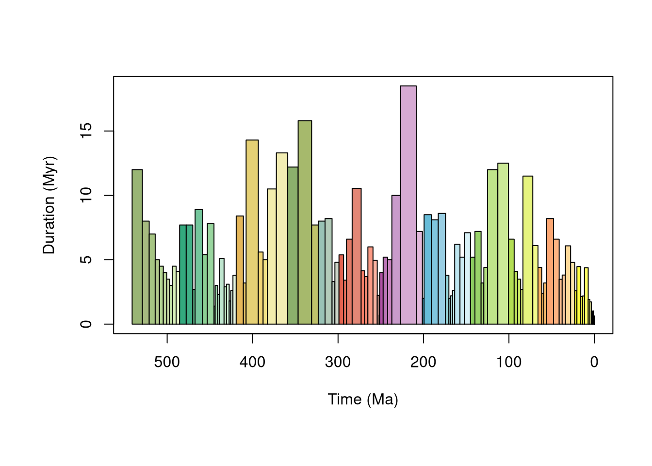
head(bins)Output
  bin interval_name  rank max_ma mid_ma min_ma duration_myr abbr  colour  font
1   1     Fortunian stage  541.0 535.00  529.0         12.0   Fo #99B575 black
2   2       Stage 2 stage  529.0 525.00  521.0          8.0   S2 #A6BA80 black
3   3       Stage 3 stage  521.0 517.50  514.0          7.0   S3 #A6C583 black
4   4       Stage 4 stage  514.0 511.50  509.0          5.0   S4 #B3CA8E black
5   5       Wuliuan stage  509.0 506.75  504.5          4.5  Wul #B3D492 black
6   6       Drumian stage  504.5 502.50  500.5          4.0   Dr #BFD99D black
Now we have our time bins, we can start to think about how we want to bin our data, but first, let’s do a little bit of housekeeping to streamline our subsequent code:
# Now we have numeric ages for our data, we can
# remove pre-Phanerozoic data to fit study scope
reefs <- subset(reefs, interval_max_ma <= max(bins$max_ma))
# bin_time() defaults to "max_ma" and "min_ma" columns
# Rename columns in reefs
colnames(reefs)[which(colnames(reefs) == "interval_max_ma")] <- "max_ma"
colnames(reefs)[which(colnames(reefs) == "interval_min_ma")] <- "min_ma"
Five methods exist in bin_time() for binning occurrence data. You can see details on each via ?bin_time:
# Bin by midpoint age
bin_time(..., method = "mid")
# Bin by overlap majority
bin_time(..., method = "majority")
# Bin into every bin within age range
bin_time(..., method = "all")
# Bin randomly into bins within age range (equal probability)
bin_time(..., method = "random", reps = 100)
# Bin randomly into bins within age range (uniform probability)
bin_time(..., method = "point", reps = 100)
CautionExercise 4: Choose a temporal binning method
Before we pick a method, let’s see how the choice impacts the data.
# Your turn: bin `reefs` using different methods
bin_time(reefs, max_ma = ___, min_ma = ___, bins = ___, method = ___)- Which method increases the number of rows?
- Which method(s) return a
list? Why? - How many occurrences remain if we use
method = "majority"and filter overlap percentage to more than 50% (hint: “overlap_percentage” column)?
TipExercise 4: Answers
-
"all": This method bins an occurrence into every bin its age range covers. For occurrences with age ranges of more than one bin, the occurrence row is duplicated. -
"random"and"point": These methods sample ages randomly so the bin assignment can differ from run to run. Therepsargument repeats sampling (e.g.reps = 100) and the output list is of lengthreps, with one binned dataset per replicate. Seehelp(bin_time)for further details. - 3946
For this tutorial, we will go with "all", which essentially generates pseudo-occurrences (similar to palaeoverse::tax_expand_time()), allowing us to count occurrences for every bin the reef potentially falls in. This is most useful for presence/absence questions (e.g. first and last appearances, range through diversity), but here we use it to offer an upper bound on where an occurrence could fall:
reefs <- bin_time(reefs, bins = bins, method = "all")Note that the number of rows of reefs has now increased: the "all" method duplicates an occurrence for every bin its age range overlaps with.
NoteHow many rows did we gain?
reefs grew from 4335 to 6554 rows. Each extra row is a copy of a reef placed in all the bins it intersects with.
Let’s check those reef numbers through time again using our binned data:
# Count number of reefs per time bin
reefs_time <- group_apply(reefs, group = "bin_midpoint", fun = nrow)
# Order chronologically
reefs_time <- reefs_time[order(as.numeric(reefs_time$bin_midpoint)), ]
# View first six rows
head(reefs_time)
Output
  nrow bin_midpoint
1    3       0.0021
2    3       0.0062
3    3      0.00995
4  117      0.07035
5   52       0.4515
6   34        1.287
That’s more like it! But let’s not forget it is always useful to visualise our data. Why don’t we plot the number of reefs through time? We can make use of the axis_geo() function to add the geological time scale to our plot:
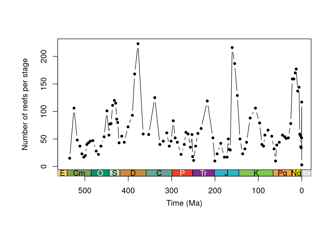
TipExercise 5: Hint
-
max()can be used to find the greatest value in a vector. -
which.max()can be used to find the row with the greatest value.
TipExercise 5: Answers
- 223
- Frasnian
TipExercise 5: Solution
   nrow bin_midpoint
72 223 377.45 bin_midpoint nrow bin interval_name rank max_ma min_ma duration_myr abbr
57 377.45 223 31 Frasnian stage 382.7 372.2 10.5 Fr
colour font
57 #F2EDAD blackYou would (and should) of course want to explore your data a little more than this. However, for brevity, let’s focus on our research theme: latitudinal trends in Phanerozoic reefs.
Palaeogeographic reconstruction
When studying modern latitudinal trends (e.g. in biodiversity), researchers can use the geographic coordinates of their samples to conduct analyses.
As the continents shift through time, palaeobiologists must reconstruct the palaeogeographic coordinates of fossil localities. To do so, Global Plate Models (e.g. PALEOMAP) are used to rotate the modern coordinates of fossil localities to their location at the time of deposition.
In palaeoverse, the palaeorotate() function allows you to do this using either the "point" or "grid" method:
-
"point": uses the GPlates Web Service to rotate point data to specific ages using the available models. -
"grid": uses reconstruction files of pre-generated palaeocoordinates (Jones and Domeier, 2024) to link the modern coordinates and age estimates of occurrences with their respective palaeocoordinates.
NoteTrade-off
The "grid" method is fast and efficient but spatially coarse (~119 km cells, so occurrences in the same cell share palaeocoordinates), while the "point" method gives higher-precision palaeocoordinates at the cost of speed, especially with many unique time intervals. The "point" method is generally preferred for fine-scale analyses or occurrences near plate boundaries.
The palaeorotate() model allows us to call multiple models at once. In this tutorial, we will use three, which lets us consider how Global Plate Model choice might impact our results: PALEOMAP, GOLONKA, and MERDITH2021 (Wright et al., 2013; Scotese & Wright, 2018; Merdith et al., 2021). For the sake of this tutorial, we will also use the "grid" method to be kind to the GPlates Web Service:
# Define the models
models <- c("PALEOMAP", "GOLONKA", "MERDITH2021")
# Palaeorotate
reefs <- palaeorotate(reefs, age = "bin_midpoint",
                      method = "grid", model = models)
Note, the first time we use palaeorotate() in each new session with method = "grid", it will take a little longer as pre-generated palaeocoordinate grids need to be downloaded from Zenodo.
# Check palaeocoordinates
head(reefs)
Output
  r_number               name             formation   system         series
1        1   Tilkideligi Tepe                       Triassic Upper Triassic
2        2              Hydra Pantokrator Limestone Triassic Upper Triassic
3        3 Shiraho, W-Pacific                        Neogene       Holocene
4        3 Shiraho, W-Pacific                        Neogene       Holocene
5        3 Shiraho, W-Pacific                        Neogene       Holocene
6        4 Aksu-Terziler area                       Triassic Upper Triassic
       interval   biota_main       biota_sec     lng    lat country
1  lower Norian Calcisponges Stromatoporoids  30.383 37.033  Turkey
2 upper Carnian       Corals    Calcisponges  23.633 37.383  Greece
3        Recent       Corals           Algae 124.250 24.333 Pacific
4        Recent       Corals           Algae 124.250 24.333 Pacific
5        Recent       Corals           Algae 124.250 24.333 Pacific
6      Tuvalian Calcisponges Stromatoporoids  31.033 37.800  Turkey
                              authors
1                          Riedel, P.
2   Schafer, P., Senowbari-Daryan, B.
3 Kayanne, H., Suzuki, A. & Saito, H.
4 Kayanne, H., Suzuki, A. & Saito, H.
5 Kayanne, H., Suzuki, A. & Saito, H.
6                          Riedel, P.
                                                                                                   title
1  Riffbiotope im Karn und Nor (Obertrias) der Tethys: Entwicklung, Einschnitte und Diversitatsmuster. -
2 The Upper Triassic Pantokrator Limestone of Hydra (Greece): An example of a prograding reef complex. -
3                       Diurnal changes in the partial pressure of carbon dioxide in coral reef water. -
4                       Diurnal changes in the partial pressure of carbon dioxide in coral reef water. -
5                       Diurnal changes in the partial pressure of carbon dioxide in coral reef water. -
6  Riffbiotope im Karn und Nor (Obertrias) der Tethys: Entwicklung, Einschnitte und Diversitatsmuster. -
  year early_stage late_stage   max_ma interval_mid_ma min_ma id n_bins
1 1990      Norian     Norian 227.0000       217.75000  208.5  1      1
2 1982     Carnian    Carnian 237.0000       232.00000  227.0  2      1
3 1995    Holocene   Holocene   0.0117         0.00585    0.0  3      3
4 1995    Holocene   Holocene   0.0117         0.00585    0.0  3      3
5 1995    Holocene   Holocene   0.0117         0.00585    0.0  3      3
6 1990     Carnian    Carnian 237.0000       232.00000  227.0  4      1
  bin_assignment bin_midpoint rot_age   rot_lng  rot_lat p_lng_PALEOMAP
1             54      217.750     218  30.00423 36.90183        21.0520
2             53      232.000     232  24.18991 37.27211        22.4745
3            100        0.010       0 124.06871 24.53673             NA
4            101        0.006       0 124.06871 24.53673             NA
5            102        0.002       0 124.06871 24.53673             NA
6             53      232.000     232  30.84884 37.82070        26.1948
  p_lat_PALEOMAP p_lng_GOLONKA p_lat_GOLONKA p_lng_MERDITH2021
1        10.0178       35.3480        8.1949           34.0895
2         2.0061       31.2992        4.3967           31.2485
3             NA            NA            NA          124.0687
4             NA            NA            NA          124.0687
5             NA            NA            NA          124.0687
6        -0.2111       37.9686        4.9978           36.2772
  p_lat_MERDITH2021 range_p_lat max_dist
1           12.1226      3.9277 1584.205
2            4.4610      2.4549 1015.764
3           24.5367          NA       NA
4           24.5367          NA       NA
5           24.5367          NA       NA
6            4.6626      5.2089 1430.176
When multiple models are called, the name of the model is added as a suffix to “p_lng_”” and ”p_lat_”.
CautionExercise 6: How far did the reefs move?
Reefs are tied to particular climatic conditions, so how much do their latitudes change once we account for plate motion? Let’s quantify it for the PALEOMAP model.
# Your turn: absolute difference between modern latitude ("lat")
# and PALEOMAP palaeolatitude, for each reef
lat_shift <- abs(reefs$___ - reefs$___)
# Mean shift across all reefs (ignore missing values)
mean(lat_shift, na.rm = TRUE)
What is the mean absolute latitudinal shift?
TipExercise 6: Hint
The modern latitude column is called lat. The palaeolatitude column from the PALEOMAP model is p_lat_PALEOMAP.
TipExercise 6: Answers
32.64 degrees
TipExercise 6: Solution
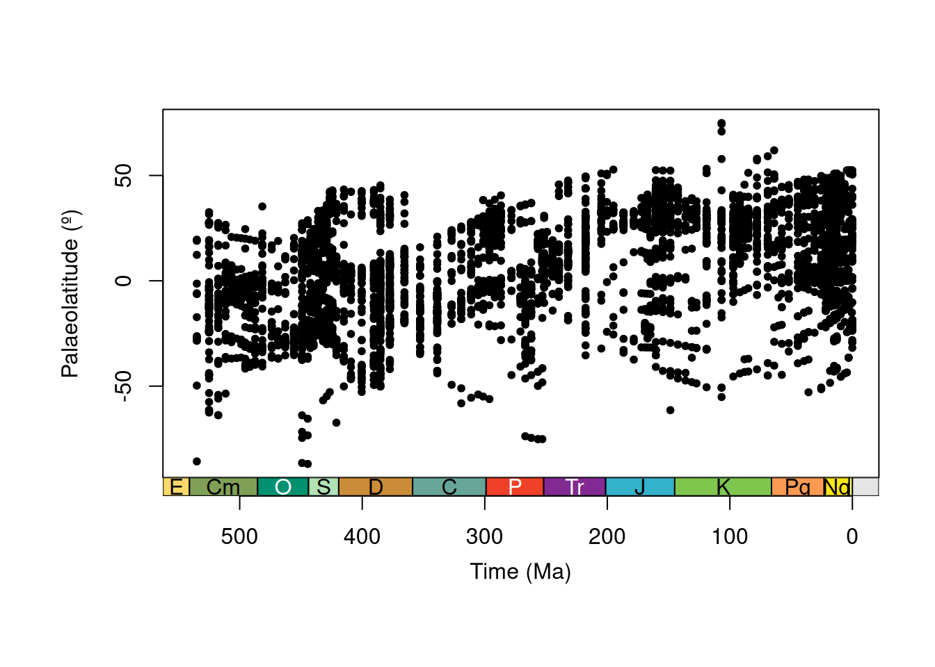
Now let’s plot that palaeolatitudinal distribution!
Summarising palaeolatitudinal trends
Neat! But it is hard to draw any trends from these data points (there are a lot of them!). We can do better by summarising this information. If we assume that reefs are broadly limited to tropical and subtropical climatic conditions, the most poleward reef in each time bin should give us an estimate of the palaeolatitudinal extent of those conditions.
# Assume hemispheric symmetry and convert
# palaeolatitudes to absolute palaeolatitudes
reefs$abs_p_lat_PALEOMAP <- abs(reefs$p_lat_PALEOMAP)
# Calculate the most poleward palaeolatitude for each time bin
paleomap_max <- group_apply(
  reefs,
  group = "bin_midpoint",
  fun = function(x) {
    data.frame(
      bin_midpoint = unique(x$bin_midpoint),
      max_p_lat = max(x$abs_p_lat_PALEOMAP, na.rm = TRUE)
    )
  }
)
# Plot data
plot(x = paleomap_max$bin_midpoint,
     y = paleomap_max$max_p_lat,
     xlab = "Time (Ma)",
     ylab = "Most Poleward Palaeolatitude (º)",
     xlim = c(541, 0),
     xaxt = "n",
     type = "b",
     pch = 20)
# Add axis of the geological time scale
axis_geo(side = 1, intervals = "periods")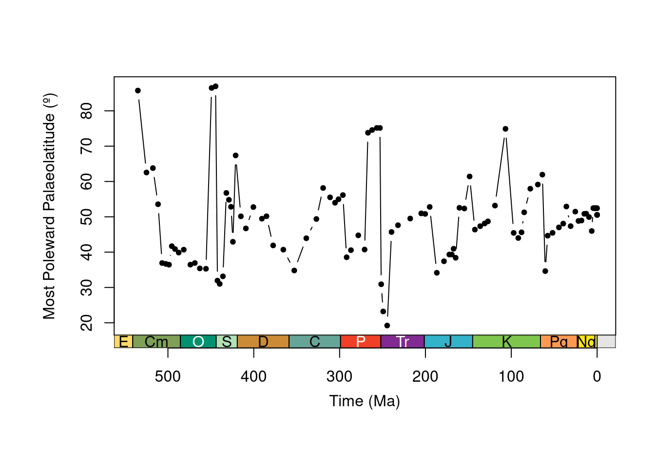
That is definitely much clearer!
Should we stop there? Well, how about one last thing: let’s repeat what we did above and calculate the most poleward reef occurrence for each of our three models and compare.
CautionExercise 7: Compare palaeogeographic reconstructions
Complete the code to calculate the most poleward palaeolatitude per bin for each model.
# Your turn: PALEOMAP has been done for you above. Now complete
# the code for GOLONKA and MERDITH2021
# Calculate the most poleward palaeolatitude for each time bin

# GOLONKA Global Plate Model
# palaeolatitudes to absolute palaeolatitudes
reefs$___ <- abs(reefs$___)
# Calculate the most poleward palaeolatitude
___ <- group_apply(
  reefs,
  group = "bin_midpoint",
  fun = function(x) {
    data.frame(
      bin_midpoint = unique(x$___),
      max_p_lat = max(x$___, na.rm = TRUE)
    )
  }
)

# MERDITH2021 Global Plate Model
# palaeolatitudes to absolute palaeolatitudes
reefs$___ <- abs(reefs$___)
# Calculate the most poleward palaeolatitude
___ <- group_apply(
  reefs,
  group = "bin_midpoint",
  fun = function(x) {
    data.frame(
      bin_midpoint = unique(x$___),
      max_p_lat = max(x$___, na.rm = TRUE)
    )
  }
)
TipExercise 7: Hint
Use the column names "p_lat_GOLONKA" and "p_lat_MERDITH2021".
TipExercise 7: Solution
# Calculate maximum palaeolatitude of reefs for each time bin for each model

# GOLONKA Global Plate Model
# palaeolatitudes to absolute palaeolatitudes
reefs$abs_p_lat_GOLONKA <- abs(reefs$p_lat_GOLONKA)
# Calculate the most poleward palaeolatitude
golonka_max <- group_apply(
  reefs,
  group = "bin_midpoint",
  fun = function(x) {
    data.frame(
      bin_midpoint = unique(x$bin_midpoint),
      max_p_lat = max(x$abs_p_lat_GOLONKA, na.rm = TRUE)
    )
  }
)

# MERDITH2021 Global Plate Model
# palaeolatitudes to absolute palaeolatitudes
reefs$abs_p_lat_MERDITH2021 <- abs(reefs$p_lat_MERDITH2021)
# Calculate the most poleward palaeolatitude
merdith2021_max <- group_apply(
  reefs,
  group = "bin_midpoint",
  fun = function(x) {
    data.frame(
      bin_midpoint = unique(x$bin_midpoint),
      max_p_lat = max(x$abs_p_lat_MERDITH2021, na.rm = TRUE)
    )
  }
)
Now, let’s plot to compare:
# Set up plot
plot(x = NULL,
     y = NULL,
     xlab = "Time (Ma)",
     ylab = "Palaeolatitude (º)",
     xlim = c(541, 0),
     ylim = c(0, 90),
     xaxt = "n")
# Plot maximum palaeolatitudes for each model
lines(x = paleomap_max$bin_midpoint, y = paleomap_max$max_p_lat,
      type = "o", col = "#e41a1c", pch = 15)
lines(x = golonka_max$bin_midpoint, y = golonka_max$max_p_lat,
      type = "o", col = "#377eb8", pch = 16)
lines(x = merdith2021_max$bin_midpoint, y = merdith2021_max$max_p_lat,
      type = "o", col = "#4daf4a", pch = 17)
# Add legend
legend(535, 20, legend = c("PALEOMAP", "GOLONKA", "MERDITH2021"),
       col = c("#e41a1c", "#377eb8", "#4daf4a"),
       lty = 1, pch = c(15, 16, 17), bty = "n")
# Add geological time scale axis
axis_geo(side = 1, intervals = "periods")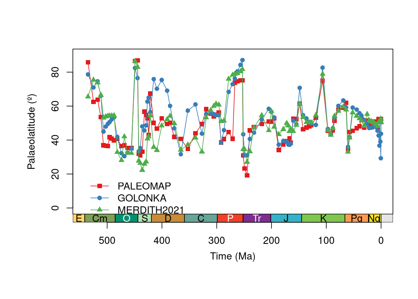
What can you observe from this plot? You may want to think about:
- Which intervals are most different?
- Where do trends converge and diverge?
- Can we reliably identify any long-term trends?
- What could we do next with this data?
We will leave you to make your own conclusions from here!
Wrap-up
Hopefully this tutorial has shown you some of the potential uses of palaeoverse functions and helped provide a workflow for your own analyses.
In this tutorial, you have:
- explored an occurrence dataset and run functions across groups with
group_apply() - linked interval names to a common time scale with
look_up() - binned occurrences with
time_bins()andbin_time() - estimated palaeocoordinates with
palaeorotate() - compared how Global Plate Model choice impacts your results
References
Buffan, L., Jones, L. A., Domeier, M., Scotese, C. R., Zahirovic, S., & Varela, S. (2023). Mind the uncertainty: Global plate model choice impacts deep‐time palaeobiological studies. Methods in Ecology and Evolution, 14(12), 3007-3019. DOI: 10.1111/2041-210X.14204.
Jones, L. A., Domeier, M. A Phanerozoic gridded dataset for palaeogeographic reconstructions. Scientific Data 11, 710 (2024). DOI: 10.1038/s41597-024-03468-w.
Kiessling, W. (2001). Paleoclimatic significance of Phanerozoic reefs. Geology, 29, 751–754. DOI: 10.1130/0091-7613(2001)029%3C0751:PSOPR%3E2.0.CO;2.
Kiessling, W. & Krause, M. C. (2022). PaleoReefs Database (PARED) (1.0) [Data set]. DOI: 10.5281/zenodo.6037852.
Merdith, A., Williams, S. E., Collins, A. S., Tetley, M. G., Mulder, J. A., Blades, M. L., Young, A., Armistead, S. E., Cannon, J., Zahirovic, S., & Müller, R. D. (2021). Extending full-plate tectonic models into deep time: Linking the Neoproterozoic and the Phanerozoic. Earth-Science Reviews, 214, 103477. DOI: 10.1016/j.earscirev.2020.103477.
Perrin, C. & Kiessling, W. (2010). Latitudinal trends in Cenozoic reef patterns and their relationship to climate. Carbonate Systems during the Oligocene–Miocene Climatic Transition, 17–33. DOI: 10.1002/9781118398364.ch2
Scotese, C. & Wright, N. M. (2018). PALEOMAP Paleodigital Elevation Models (PaleoDEMs) for the Phanerozoic. PALEOMAP Project.
Wright, N., Zahirovic, S., Müller, R. D., & Seton, M. (2013). Towards community-driven paleogeographic reconstructions: integrating open-access paleogeographic and paleobiology data with plate tectonics. Biogeosciences, 10(3), 1529–1541. DOI: 10.5194/bg-10-1529-2013.
Session info
─ Session info ───────────────────────────────────────────────────────────────
 setting  value
 version  R version 4.6.2 (2026-10-29)
 os       Ubuntu 26.04.1 LTS
 system   x86_64, linux-gnu
 ui       X11
 language (EN)
 collate  C.UTF-8
 ctype    C.UTF-8
 tz       UTC
 date     2026-11-19
 pandoc   3.7.0.2 @ /usr/bin/pandoc
 quarto   1.11.9 @ /usr/local/bin/quarto

─ Packages ───────────────────────────────────────────────────────────────────
 ! package     * version date (UTC) lib source
   ape           5.8-1   2024-12-16 [1] RSPM
   askpass       1.2.1   2024-10-04 [1] RSPM
   class         7.3-24  2026-08-03 [2] CRAN (R 4.6.2)
   classInt      0.4-11  2025-01-08 [1] RSPM
   cli           3.6.6   2026-04-09 [1] RSPM
 R cpp11         <NA>    <NA>       [?] <NA>
   curl          8.1.0   2026-10-14 [1] RSPM
   DBI           1.3.0   2026-02-25 [1] RSPM
   digest        0.6.39  2025-11-19 [1] RSPM
   dplyr         1.2.1   2026-04-03 [1] RSPM
   e1071         1.7-17  2025-12-18 [1] RSPM
   generics      0.1.4   2025-05-09 [1] RSPM
   geojsonsf     2.0.5   2025-11-26 [1] RSPM
 R geometries    <NA>    <NA>       [?] <NA>
   geosphere     1.6-8   2026-04-05 [1] RSPM
   glue          1.8.1   2026-04-17 [1] RSPM
   h3jsr         1.3.1   2023-01-21 [1] RSPM
   httr          1.4.9   2026-09-01 [1] RSPM
 R jsonify       <NA>    <NA>       [?] <NA>
   jsonlite      2.0.0   2025-03-27 [1] RSPM
   KernSmooth    2.23-27 2026-08-12 [2] CRAN (R 4.6.2)
   lattice       0.23-1  2026-08-12 [2] CRAN (R 4.6.2)
   lifecycle     1.0.5   2026-01-08 [1] RSPM
   magrittr      2.0.5   2026-04-04 [1] RSPM
   mime          0.13    2025-03-17 [1] RSPM
   nlme          3.1-171 2026-09-01 [2] CRAN (R 4.6.2)
   openssl       2.6.0   2026-11-17 [1] RSPM
   palaeoverse   1.5.0   2026-06-11 [1] RSPM
   pbapply       1.7-5   2026-09-01 [1] RSPM
   pillar        1.11.1  2025-09-17 [1] RSPM
   pkgconfig     2.0.3   2019-09-22 [1] RSPM
   proxy         0.4-29  2025-12-29 [1] RSPM
   purrr         1.2.2   2026-04-10 [1] RSPM
   R6            2.6.1   2025-02-15 [1] RSPM
 R rapidjsonr    <NA>    <NA>       [?] <NA>
   Rcpp          1.1.2   2026-07-05 [1] RSPM
   rlang         1.3.0   2026-07-05 [1] RSPM
   s2            1.1.13  2026-09-28 [1] RSPM
   sf            1.1-3   2026-09-11 [1] RSPM
 R sfheaders     <NA>    <NA>       [?] <NA>
   stringdist    0.9.17  2026-01-16 [1] RSPM
   stringi       1.8.9   2026-08-04 [1] RSPM
   stringr       1.6.0   2025-11-04 [1] RSPM
   sys           3.4.3   2024-10-04 [1] RSPM
   tibble        3.3.1   2026-01-11 [1] RSPM
   tidyr         1.3.2   2025-12-19 [1] RSPM
   tidyselect    1.2.1   2024-03-11 [1] RSPM
   units         1.0-1   2026-03-11 [1] RSPM
   utf8          1.2.6   2025-06-08 [1] RSPM
   V8            8.2.1   2026-10-26 [1] RSPM
   vctrs         0.7.3   2026-04-11 [1] RSPM
   withr         3.0.3   2026-06-19 [1] RSPM
   wk            0.9.5   2025-12-18 [1] RSPM

 [1] /home/runner/work/_temp/Library
 [2] /opt/R/4.6.2/lib/R/library

 R ── Package was removed from disk.

──────────────────────────────────────────────────────────────────────────────